This blog post is based on the net surgery example provided by Caffe. It takes the concept and expands it to a working example to produce pixel-wise output images, generating output in ~2 seconds (simple approach) or ~35 seconds (advanced approach) for a 2,000 x 2,000 image, an improvement from the  ~15 hours of a naive pixel wise approach.

Introduction

The net surgery example discusses how to take a patch level classifier and convert it to a fully convolutional network. The underlying concept is that convolutions are agnostic to the input size, but that the fully connected layers need to be modified such that they can be computed in a convolutional fashion. This is done by modifying both the deploy file and the associated Caffe model.

Here we present two approaches. A fast (simple) approach which runs the classifier once across the image and uses it to interpolate the necessary pixel values to generate a full size image pixel wise image. The second (advanced) approach runs the DL classifier multiple times at different displacement offsets to generate a very accurate image. While the computational cost is higher (35 seconds vs 1.5 seconds), it is still a far cry from the original 15 hours it would take to perform the same operations pixel-wise.

Architecture Constraints

The network architecture used for this process cannot have any padding at any of the levels. This should make some intuitive sense. As we’re operating on the whole image at a single time, the only padding which would take place are at the absolute edges. When operating at the patch level, the padding occurs on the edges of every patch, providing either 0’s or mirrored pixels (in the case of caffe the padding style is 0s).

The easiest way to check is by using grep:

If there is no output, then no padding variables are set, and we should be good to go!

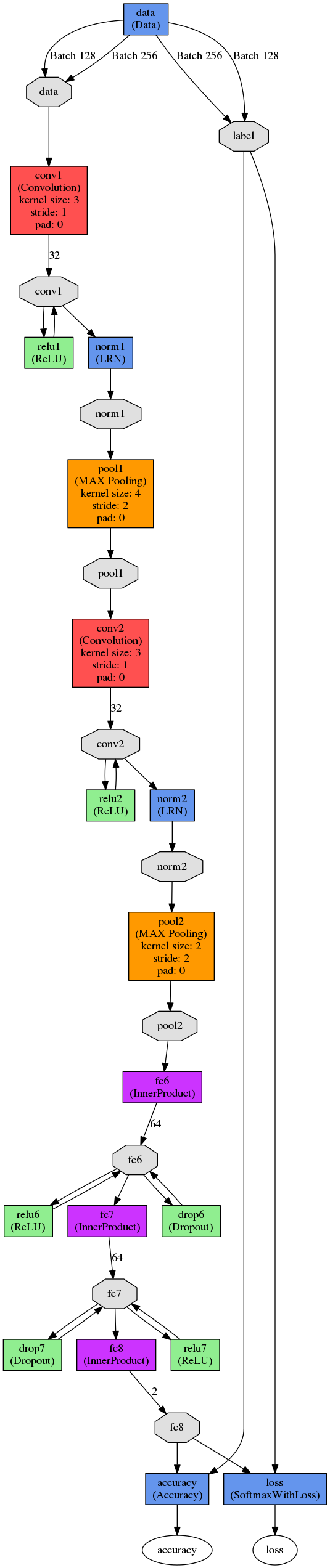
Here is an example of the network we’re using, note the lack of padding (click for large version):

Conversion

We use the same process as described in the net surgery example, and explicitly state each of the steps.

1. Copy the deploy.prototxt to a deploy_full.prototxt
2. Identify all InnerProduct layers, in this case, fc6, fc7 fc8:

Replace all instances of the layer name with an appended “-conv”, e.g., fc6 -> fc6-conv, fc7 -> fc7-conv, etc. This prevents Caffe from accidentally loading the old values from the model file and more accurately represents the layer type (remember, we’re converting them from fully connected to convolutional).

3.  Replace “InnerProduct” with “Convolution”

4. Replace “inner_product_param” with “convolution_param”

5. Add “kernel_size: 1″ to convolutional_param for all these layers except for the first layer we’re changing (i.e., fc6-conv).

6. Fc6-conv is a bit trickier to figure out, we need to know the exact size of the kernel which comes in. This is trivially done if we look at the training log from the patch level classifier, as it states the input and output sizes of each layer as it scaffolds them:

Here we can that the top shape is 128 x 32 x 6 x 6. 128 is our batch size, 32 is the num_output from the previous convolution later, leaving us with a 6 x6 kernel. As a result, we set fc6-conv “kernel_size: 6”.

7. We need to specify the exact input size of the image we’ll be using, otherwise Caffe will resize (and possibly change the aspect ratio) the size of our input image to the specification size. In this case, we had a 32 x 32 patch classifier, and we want to use it on 2032 x 2032 images, so we modify the deploy file accordingly:

Note that our actual input image is 2000 x 2000, except we want to be able to compute the edges, so during output generation time we’ll mirror the edges by exactly half the patch size. In this case, that comes to +16 pixels on each size.

8. Depending on the method used to make the deploy file (such as NVIDIA Digits) , we may need to add the bottom softmax layer to get a probability distribution, this is done by simply adding to the bottom of the file:

With that information, we can use convert-patch-classifier-to-full-convolutional.py to make a new caffe model for us. Here we can see the old and new deploy models.

Output Generation (Simple)

Using our new network, we simply need to feed the image into the classifier and get the output. Note that the size of the image is 2000 x 2000, we specified a padded size of 2032 x 2023 above in the deploy text. The padding occurs in cell [6]. These sizes need to be the same!

We can see the code in action here.

Here we note two thing, first off, we’ve produced our input image in ~2 seconds. Not bad!

Secondly, we can see that the intermediate output image (im_out) is actually of size 501 x 501 and not the 2000 x 2000 we expected. This makes some sense, since at each layer we reduce the data size through convolution and pooling. The python script takes these values and interpolates them correctly back to the larger image.

Depending on your image size and network characteristics, this is a critical step. We define what we call the “image_ratio”, which is the ratio from the larger image to the smaller image, in this case 2000 x 501 = 3.992.

Since this image ratio is not an integer (and can be “worse” such as 3.5), it has a compounding effect on the pixel location in im_out versus im_out_final. For example, if we have an output image of 500 x 500, the image ratio would put the 500th pixel at 500 * 3.99 = 1995. When, we know for a fact that it comes from an image of 2000 x 2000. We can see that as the images get larger the image ratio introduces more and more error, in this case, the pixel is incorrectly located 5 pixels away from its “real” location. This is why the interpolation is so important!

Below we can see the result from a nuclei segmentation task, as generated by this new efficient code (left) versus the pixel-wise naive approach (right). Looking nearly identical, but with 99.996% less computation time!

Output Generation (Advanced)

At this point, we already have a very rapid output generation approach, but we’re not really computing the network at each pixel. In effect we’re computed every image_ratio pixel and interpolating the ones in between. While this is more than sufficient in most cases, is it possible to compute the pixels in between and interlace them in an efficient manner? It certainly is 🙂

If we know our image_ratio, we can displace the original image inside of this “receptive field“, compute output at each displacement, and then merge them together. More explicitly, compute row/column displacements of image_ratio. In this case, that’s operations. If each operation took ~2 seconds before, we’d expect to get them all done in ~30 seconds. Still pretty impressive!

At a high level the results look the same between the two methods, but if we zoom in on a 288 x 271 region, we can see some striking differences:

Simple Approach

Advanced Approach

Where the left image shows the overlay of the right image on this original image

We can see the code in action here.

That pretty much sums it up! The entire code base is available here.