Deep learning (DL) models have been performing exceptionally well on a number of challenging tasks lately. Unfortunately, given the current blackbox nature of these DL models, it is difficult to try and “understand” what the network is seeing and how it is making its decisions. Building upon our previous post discussing how to train a DenseNet for classification, we discuss here how to apply various visualization techniques to enable us to interrogate the network. The code here is designed as drop-in functionality for any network trained using the previous post, hopefully easing the burden of its implementation.

To test the validity of these approaches, it is often easier to create a synthetic dataset with known properties before translating the technology to the target domain. In this case, we use make_hdf5_synthetic_circles_and_boxes.ipynb to generate data for a 2 class task of identifying if the image contains a square or does not contain a square:

 

Negative Class

Positive Class

 

This straightforward task should be ideal for evaluating visualization approaches since we would expect the areas of interest to be around the square, if one is present. To proceed, we need to train a network, which we do with the train_densenet.ipynb. This approach follows along with the previously presented training approach. Once the training is done, we can begin with the visualizations.

Looking at visualizations

The code begins by extracting an image from the positive class. Here we can see that it belongs in the positive class because there is a square present:

For simplicity, we don’t perform any preprocessing besides cropping the image to the appropriate size and converting it from a nrow x ncol x ndim image to a ndim x nrow nxcol tensor in the range of [0,1].

We evaluate the image using the model and see that the correct class is in fact predicted. Off to a good start!

 

To perform the visualizations we use the follow code from utkuozbulak on github. The methods discussed below are, Vanilla backpropogation, Guided backpropogation, GradCam, and Guided GradCam. Note that here we only briefly introduce each approach and show an example of its output. The original github repository contains in-depth references which should be reviewed for a deeper understanding of the approaches. Additionally, that code has been modified slightly to work with DenseNets (as opposed to VGG) and to also work using the GPU. A CPU can also be used, as there is not a notable amount of computation required to generate these results.

Vanilla Backpropagation: apply model to image, set class of interest, backprop to compute gradient with respect to specified class. Here we can see a 3×3 grid of output from this process:

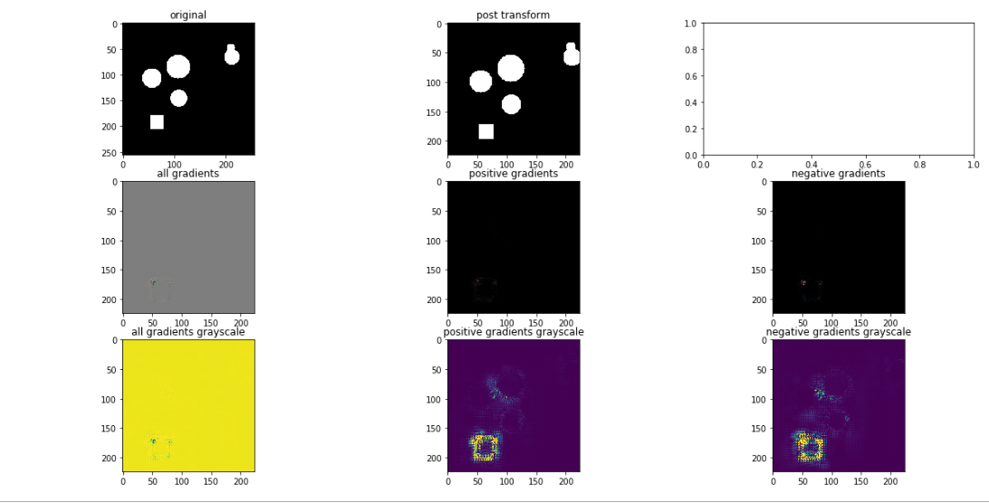
Top row: original image, post-transformed image (in case we do augmentation, to see what actually goes “into” the network), an extra plot (ignore)

Middle row: All gradients implies seeing gradients which are both positive an negative. Positive gradients highlights positive gradients (tends to indicate pixels important for identifying a class). Negative gradients highlights pixels which tend to relate to other classes besides the chosen one.

Bottom row: same as middle row except with preferable scaling. This scaling essentially caps outliers so the “visible” range is more realistic and visually useful.

We can see that this approach successfully identifies the edges of the square, which one can think of as the most defining characterization of the positive class. Note as well that the negative class isn’t too impressive here, likely as a result of this being a trivial use case. With additional complexity, and classes (>2), these negative images are likely to become more interesting and differentiate themselves from the positive class.

Guided Backpropagation: apply model to image, set class of interest, backprop to compute gradient with respect to specified class. Except that this time during the backpropagation process, replace all gradients which are less than 0 with 0. This has been shown to more aggressively focus the visualization signal:

 

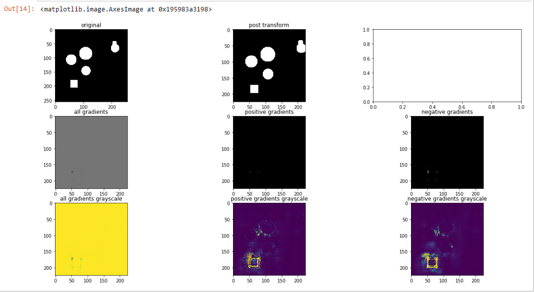
We can see that in fact, the edges are a bit crisper around the square. Interestingly, we can start to see a faint border around the circle.

GradCam: this is a more sophisticated approach which allows for a highlighting of the region of interest. This tends to be more easily interpretable and less noisy than solely examining individual pixels.

We show the outputs from using GradCam on each layer, starting at the first layer and proceeding left to right, and up to down, where the last layer is in subplot (3,3).

Note that typically one only looks at the last layer of Gradcam, but here we show all layers as it may be interesting to note where certain regions start to become filtered out.

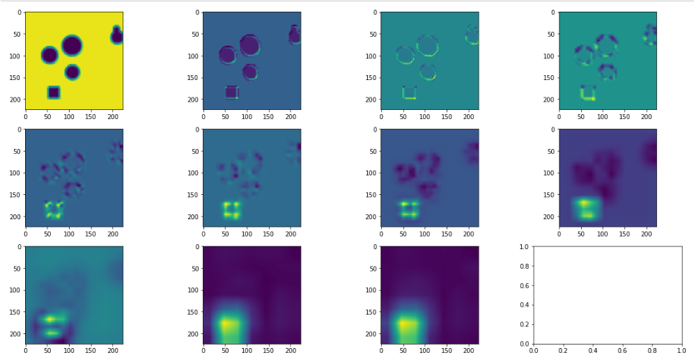
We can see here again that the square region is quite readily identified, though in a more smoothed manner. Interestingly, it seems that the upper left corner is, in fact, a stronger driving force than any other section of the square.

Guided GradCam: essentially a synergistic combination of both Guided backpopogation and Gradcam. Again, only the last layer tends to be relevant, but the additional layers are provided for completeness. We can see here the best result so far, where the square is precisely delineated, indicating that it was the driving force in determining that this image belongs to the positive class.

 

Conclusion

While these results are encouraging, they should be taken with a grain of salt and modest skepticism. Although they give us hints as to what the DL model may be using to make its decisions, we must beware of our own positive confirmation biases. A worthwhile easily approachable discussion of that is presented here.

To add on in the context of this use case, just because we are highlighting the square, does not indicate that the system knows precisely what a square is. For example, it looks like these filters are highlighting straight edges; what if instead the image contained simply a line? Would that be sufficient to cause a positive class, and if it did, does that mean that we really don’t have a square detector but instead have an edge detector?

Additionally, do we have any guarantee from the information shown above that the network is not performing the classification solely based on size? This test image seems to show that the square is the smallest thing in the image, are all the squares in the training set always smaller than the rest of the circles? Did we simply make a “small” object detector?

Keep in mind that this dataset and task is extremely trivial, one can imagine how in a real-world situation the space of potential “explanations” for the model would be exponentially larger (light/hue characteristics, texture, etc). So, just because we’re getting the results we’re expecting, doesn’t imply that we’re getting them for the reasons that we think we are.

If anything, these approaches are solely providing a direction of inquiry for future testing!

All code available here